LAB #6

LAB #7

CSC 101
Introduction to Spreadsheets

R Mohammadi

October 1998
Objectives:

Learn more about the tools offered by Microsoft Excel.

Learn about functions and addressing in spreadsheets.

about this lab ...

You will need your 3.5" disk for this lab and you must have completed lab#6 and already have a lab6 file on your disk. As always, you will also need your MS office Starts Here CD.

1. Learn to calculate values and format Excel workbooks with Microsoft Office Starts Here.

Place your CD for Microsoft Office Starts Here in your CD-ROM Drive. Click the Quit button if a dialog box comes up to auto-start the software.

Start Microsoft Office Starts Here by clicking the Icon on your desktop.

Choose the Basics by clicking on it.

On the left hand side of the Window under Sections, pick

Do the two lessons, Calculate Values and Format a worksheet.

Take Quiz after each lesson. Be sure to let your lab instructor see the results before you continue.

Close the window by clicking on the X in its upper right hand corner.

2. Starting Microsoft Excel.

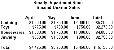
Start Microsoft Excel by clicking on Start, clicking on Programs, and then clicking Microsoft Excel. An Excel window should be on your screen.

3. Enter 3^rd and 4^th Quarter tables.

Open the Excel file from lab6. The following worksheet should appear on your screen:

	Smally Department Store
	First Quarter Sales

	January	February	March	Total
Clothing	$1,500.00	$1,600.00	$1,800.00	$4,900.00
Toys	$ 800.00	$ 700.00	$ 800.00	$2,300.00
Houseware	$1,200.00	$1,600.00	$1,700.00	$4,500.00
Jewelry	$ 900.00	$1,100.00	$ 700.00	$2,700.00

Total	$4,400.00	$5,000.00	$5,000.00

Copy and paste these tables in creating the 3^rd and the 4^th quarter sales tables for our store. The 3^rd and 4^th quarter sales tables must appear below the first two in the correct sequence. You should only have to change the header and the individual sales values for the new tables as the formulas will be inherited. The new tables should be as follows:

	Smally Department Store
	Third Quarter Sales

	July	August	September	Total
Clothing	$ 750.00	$ 875.00	$1,000.00	$2,625.00
Toys	$ 387.50	$ 375.00	$ 375.00	$1,137.50
Houseware	$ 650.00	$ 875.00	$ 900.00	$2,425.00
Jewelry	$ 425.00	$ 500.00	$ 450.00	$1,375.00

Total	$2,212.50	$2,625.00	$2,725.00


	Smally Department Store
	Forth Quarter Sales

	October	November	December	Total
Clothing	$2,250.00	$2,625.00	$3,000.00	$7,875.00
Toys	$1,162.50	$1,125.00	$1,125.00	$3,412.50
Houseware	$1,950.00	$2,625.00	$2,700.00	$7,275.00
Jewelry	$1,275.00	$1,500.00	$1,350.00	$4,125.00

Total	$6,637.50	$7,875.00	$8,175.00

4. Change Table colors.

For each table,

highlight the complete table

in the Format menu, choose Cells… You should now see the Format Cells pop-up window.

Click the Pattern tab.
Choose a color (a different color for each table) and click the OK button.

5. Develop a summary table.

We want a table that only reports the totals for the different items in each quarter; however, we don't wish to reenter all those totals again. You may think that you could copy/paste the totals into the new table from each of the four tables, but the cell series that SUM functions apply to will actually change when you copy /paste. Here is what would work best in this case:

Type in the header/labels for the summary table as shown below, to the right of the original 4 tables.

Make Q1/Clothing cell in the Summary table reference the Total/Clothing cell of the 1^st quarter table. In the intersection Q1 and Clothing, type =E5, assuming E is the column for Total of the 1^st quarter table and 5 is the row for clothing in the 1^st quarter table. Don't just type =E5, make sure you reference the correct cell.

Repeat this process for the Q2/Clothing using the Total/Clothing cell in the 2^nd quarter table.

Repeat this process for the Q3/Clothing using the Total/Clothing cell in the 3^rd quarter table.

Repeat this process for the Q4/Clothing using the Total/Clothing cell in the 4^th quarter table.

Highlight all data cells for the summary tables and in the Edit menu, choose Fill, in the Fill submenu, choose down. You should have the following table:



	Smally Department Store
	Sales Summary
	Q1	Q2	Q3	Q4	Total

Clothing	$4,900.00	$5,250.00	$2,625.00	$7,875.00
Toys	$2,300.00	$2,275.00	$1,137.50	$3,412.50
Houseware	$4,500.00	$4,850.00	$2,425.00	$7,275.00
Jewelry	$2,700.00	$2,750.00	$1,375.00	$4,125.00

Total

Highlight the cells starting with the intersection of Q1 and Clothing until row and column Total cells.

Click the Sum button, this will automatically fill in all totals cells in this table. You will have to widen your columns for the totals to fit, notice that the totals will appear as a sequence of ####s. Point to the line separation between column labels on top of the worksheet, press left mouse button and drag, to the right, you should notice the column getting wider. The columns only need to be slightly wider for the total values to be visible.

6. Why all this fuss.

The key reason for implementing summary tables in this way is that if the data changes in the detail tables, without any work from the user (you) the summary data is updated appropriately. Try changing Clothing sales in June or Jewelry sale in September, you will notice that their summary data changes accordingly. Be sure to let your lab instructor see your worksheet.

7. Save your spreadsheet.

Save this sheet as LAB7 on your 3 ½" Floppy (A:). You have now completed the lab. Logout of the workstation after your lab instructor examines your work.